The power of predicate pushdown

In our last article we provided an overview of the inner workings of Polars. In this blog we will dive into the query optimizer and explain how one of the most important optimization rules works: predicate pushdown. The idea is simple yet effective, apply any filters you have as close to the data source as possible. This avoids unnecessary computation for data that will be thrown away and reduces the amount of data being read from disk or send over the network. Note that predicate pushdown (and all other optimizations) happen under the hood automatically.

What is a predicate? A predicate in the context of data processing refers to a filter or condition which is imposed on the data usually in the form of a boolean expression, e.g. column_a > 2. A row for which the condition does not evaluate to true is discarded.

Simple Example

Let us start with a simple example to show the concept of a predicate. Later on we will work our way through more common enterprise cases. Say we have a simple CSV net_worth.csv:

age,net_worth
1,0
30,50000
50,60000
70,100000

And we wish to calculate the average net_worth of people above the age of forty:

df = (
    pl.scan_csv("net_worth.csv")
    .filter(pl.col("age") > 40)
    .select(pl.col("net_worth").mean())
)
df.show_graph(optimized=False)

The computation graph is best read from bottom to top as data is passed from the leaf nodes to the root.

If we look at the unoptimized computation graph we can see that the filter is the first computation done on the dataset. Great! But we can do even better. We first read in the entire CSV and then discard any data we don’t need. For larger files, this can become memory intensive. A better approach would be to apply our filter immediately when reading in the data, removing the need to have the entire dataset in memory at once. During the query optimization step, our query engine collects all the predicates and passes them to our IO readers.

df.show_graph(optimized=True)

For the CSV file format this means we can discard rows as we read them. However, in other cases the speed-up can even more impactful, skipping over entire memory regions or files altogether. We will discuss these in the next sections.

Parquet

In the CSV example we still have to read the entire file, in the parquet file format we can do lot better. Parquet is a complicated file format, explaining it could be multiple blogs on its own. For this blog we will zoom out a little bit and use the following structure¹.

A parquet file can roughly be divided into three sectors: a header, the data and the metadata. Data is saved in groups of rows (named row groups) and within a row group each column is saved back to back. The last sector contains metadata of the row groups. For each column in a row group we can save certain information such as the minimum & maximum value in the group column or other statistics.²

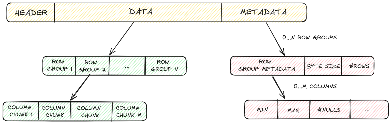
A common pattern when applying predicate pushdown in parquet files is to read the file in two steps. First you get the metadata section. Then you use your predicate to determine if a certain row group needs to be read or not. For the example column_a > 2 the parquet reader would read the column metadata of column_a and look at its min and max values for each row group. If the predicate evaluates to false then there is no need to read in the row group.

This way we can skip entire memory sections of the parquet file. This is much better than our CSV example where we had to read the entire file, here we only need to read the relevant memory regions.

In parquet, a dataset is usually spread over multiple files. For each file we still need to read the metadata which can be slow³, especially if you have many small parquet files. With hive partitioning we can do even better.

Hive Partitioning

Hive Partitioning is a simple yet powerful technique where data stored on disk is partitioned into multiple files & folders depending on values in certain key columns. The data engineer upfront decides on what these key columns are, for example splitting your dataset on time.

In the example below we split our data on the country column and put all the data which belongs to a certain country in (a) separate parquet file(s). In Hive partitioning, you (mis)use the path of the file to indicate the value for the key columns. In this case an example path could be /datawarehouse/dataset/country=USA.parquet.

In predicate pushdown, we can use this information to determine if we need to read the file at all, skipping the need to read the metadata. If used correctly, this can be extremely powerful. In the example below we query a dataset hive partitioned on countries. The logs show 192 countries could directly be skipped during reading leading to significant performance speedups.

The downside of hive partitioning is that the pushdown only works for the key columns chosen upfront. Filtering on another column would not have worked.

pl.scan_parquet("./dataset/country=*/*.parquet").filter(pl.col("country") == "GB").collect()

S3 Select

Note: at the time of writing this blog, S3 select is still in its infancy with some important restrictions, most notably the lack of parquet output support.

If you recall our mantra of applying the filter as close to the source as possible, then S3 select would be the next level. S3 is a cloud object storage by AWS which is often used in datalake solutions to store the underlying data. In the examples above (except for hive partitioning) we are still transferring the data over the network from S3 to our compute. Although network connections have gotten a lot better, it would be better if we skip transferring the data we don’t need.

This is where S3 Select comes in. As a query engine you provide your predicate in a specific format and S3 select applies the filter directly on the data. This way the filter occurs on the S3 compute server which is faster than transferring the data over the network and applying the filter on our own compute server.

Conclusion

Predicate pushdown is a powerful technique to filter your data as early as possible. This avoids performing computation on data that will be thrown away later. In this blog post we have shown several key techniques in Polars which can be used to optimize your predicate pushdown usage, ultimately saving precious compute and memory resources.